Playing with raw census data

Statistics Canada publishes “public use microdata files” that contain an anonymized random sample of census responses. The most recent version available is from the 2016 census. Statistics Canada hasn’t published microdata files for the 2021 census yet. The Individuals File for 2016 is a 2.7% sample of census responses.

Getting the data

It turns out you can’t just directly download the data. Instead, you have to fill out a form with information about yourself, and wait for your request to be manually processed. The wording of the form made it sound like they were going to mail me the data on a physical medium, but luckily I got an email with instructions a few days later instead. From there, I had to create an account on a website for exchanging data with Statistics Canada, and then finally I could log in and download the data from the CRSB_ADHOC_CENSUS_PUMF depot. Note that if you order any of the PUMF products you can access all of them with your E-transfer account.

If you want to work with the data without going through that process, you can download the data from Kaggle or the Internet Archive. Note that I didn’t include documentation files with that.

Using the data

The data is stored as a single file with a record on each line. Each field is stored in a specified range of characters on each line (left padded with spaces if needed). Fields are stored next to each other, and you can only separate them with knowledge of the schema. The schema is provided in a few formats, all of which are intended for use with proprietary statistical software.

I used one of the schema files that was somewhat easy to parse to generate a CSV version of the data, which just adds a header and sprinkles in some commas on each row. I found my CSV version was a lot easier to work with using pandas. Some of the schema data is lost this way though – if you use the raw data with the intended statistical software it will be able to use the schema to automatically infer the meaning of integer values in categorical columns, unlike with a simple CSV.

The data was sampled using stratified sampling, so not all rows have the same weight. As such, you need to multiply each row by the WEIGHT column to get accurate results. You can also use the WT1-WT16 columns in place of WEIGHT to get multiple smaller random samples – the WTX columns are 0 for most rows, but correspondingly bigger on rows where they are non-zero.

I’ve done some experimenting with the data using the Python pandas library. See this notebook for the full details on how I got these results. One simple thing we can do is deterimne the total population. By adding up all the weights, we get the population of Canada on the census reference date (May 10, 2016):

>>> df = pd.read_csv("/path/to/data.csv")
>>> df["WEIGHT"].sum()
34460064.00006676

Let’s see what other columns we have available to work with:

>>> df.columns.values
array(['PPSORT', 'WEIGHT', 'WT1', 'WT2', 'WT3', 'WT4', 'WT5', 'WT6',
       'WT7', 'WT8', 'WT9', 'WT10', 'WT11', 'WT12', 'WT13', 'WT14',
       'WT15', 'WT16', 'ABOID', 'AGEGRP', 'AGEIMM', 'ATTSCH', 'BEDRM',
       'BFNMEMB', 'CAPGN', 'CFINC', 'CFINC_AT', 'CFSIZE', 'CFSTAT',
       'CHDBN', 'CHLDC', 'CIP2011', 'CIP2011_STEM_SUM', 'CITIZEN',
       'CITOTH', 'CMA', 'CONDO', 'COW', 'CQPPB', 'DETH123', 'DIST',
       'DPGRSUM', 'DTYPE', 'EFDECILE', 'EFDIMBM', 'EFINC', 'EFINC_AT',
       'EFSIZE', 'EICBN', 'EMPIN', 'ETHDER', 'FOL', 'FPTWK', 'GENSTAT',
       'GOVTI', 'GTRFS', 'HCORENEED_IND', 'HDGREE', 'HHINC', 'HHINC_AT',
       'HHMRKINC', 'HHSIZE', 'HHTYPE', 'HLAEN', 'HLAFR', 'HLANO', 'HLBEN',
       'HLBFR', 'HLBNO', 'IMMCAT5', 'IMMSTAT', 'INCTAX', 'INVST', 'KOL',
       'LFACT', 'LICO', 'LICO_AT', 'LOC_ST_RES', 'LOCSTUD', 'LOLIMA',
       'LOLIMB', 'LOMBM', 'LSTWRK', 'LWAEN', 'LWAFR', 'LWANO', 'LWBEN',
       'LWBFR', 'LWBNO', 'MARSTH', 'MOB1', 'MOB5', 'MODE', 'MRKINC',
       'MTNEN', 'MTNFR', 'MTNNO', 'NAICS', 'NOC16', 'NOCS', 'NOL', 'NOS',
       'OASGI', 'OTINC', 'PKID0_1', 'PKID15_24', 'PKID2_5', 'PKID25',
       'PKID6_14', 'PKIDS', 'POB', 'POBF', 'POBM', 'POWST', 'PR', 'PR1',
       'PR5', 'PRESMORTG', 'PRIHM', 'PWDUR', 'PWLEAVE', 'PWOCC', 'PWPR',
       'REGIND', 'REPAIR', 'RETIR', 'ROOMS', 'SEMPI', 'SEX', 'SHELCO',
       'SSGRAD', 'SUBSIDY', 'TENUR', 'TOTINC', 'TOTINC_AT', 'VALUE',
       'VISMIN', 'WAGES', 'WKSWRK', 'WRKACT', 'YRIMM'], dtype=object)

The meaning of all of those columns is documented in the handy user guide for the data.

Working with categorical data

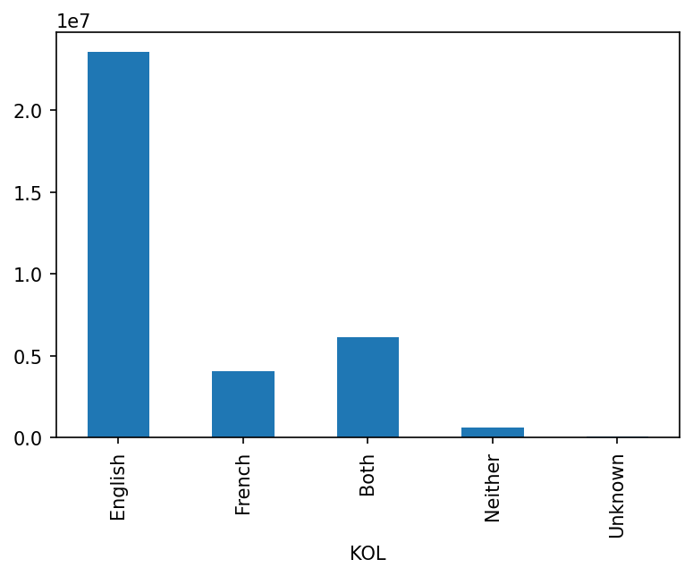
The KOL column indicates people’s Knowledge Of the official Languages of Canada (English and French). Let’s make a graph of the data:

A bar chart

Working with numberic data

The WAGES column has the total wages of respondents (according to income tax data) in Canadian dollars in 2015. According to the user guide, 88888888 and 99999999 are special values that indicate that no data is available or applicable. Let’s try making a histogram of all values with data available:

plt.suptitle("Total wages")
all_person_wages_df = df[(df["WAGES"] < 80000000)]
all_person_wages_df["WAGES"].plot(
    kind="hist", bins=250, weights=all_person_wages_df["WAGES"]
)

A histogram

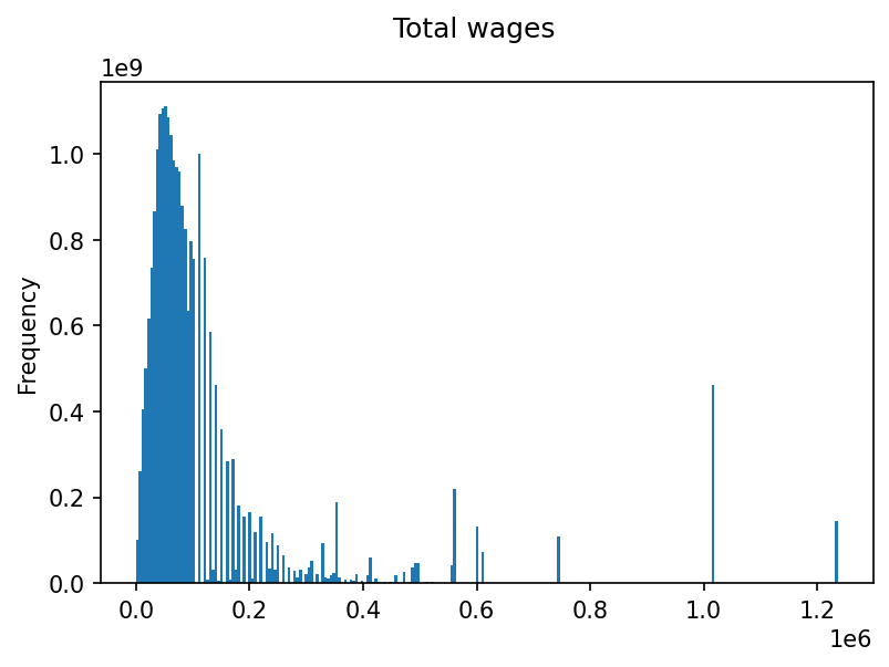
That looks weird. It appears that values above $100,000 are rounded to avoid making any rows personally identify an individual, which makes this histogram all wacky. If we change it to only plot people with total wages under $100,000 it looks fine: